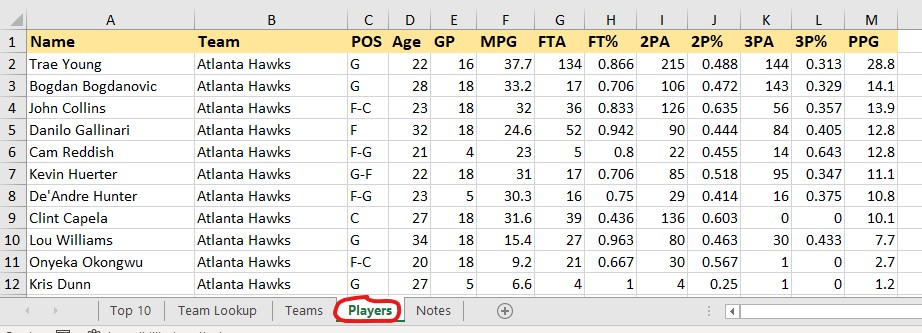
Step 1
Download the NBA.xlsx spreadsheet. It will have the Players and Notes
sheets. The Notes sheet shows the Players column abbreviations.
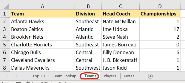
Step 2
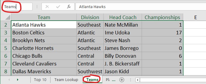
Create a new sheet named Teams. Enter all 30 NBA Teams along with the
Division, Head Coach, and number of Championships. This step may take some
time. You may want to use Wikipedia to get the information.
Step 3
Create a new sheet named Top 10. It should have the four top 10 lists as
shown.
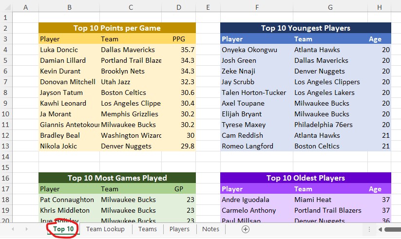
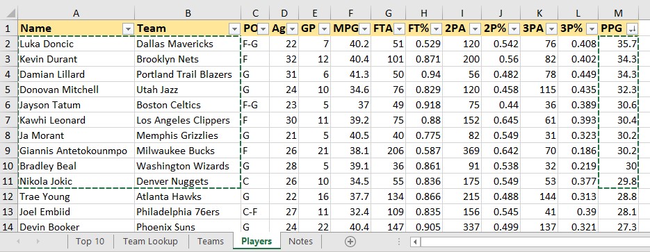
To get the Top 10 players for each category, add a filter to the Players sheet and sort it by that category.
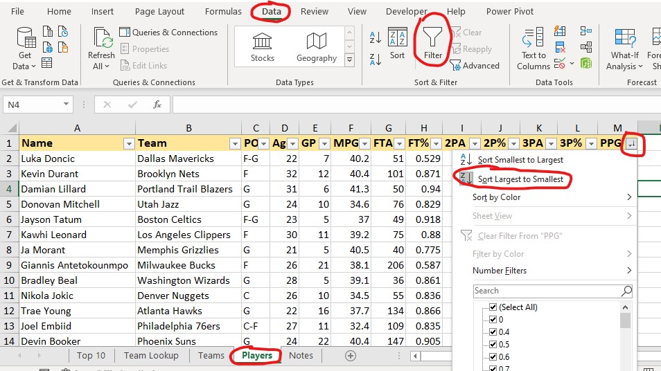
Copy & paste the Top 10 players to the Top 10 sheet. Select the top 10 players Name, Team, and PPG - hold the Ctrl key to select non-adjacent cells.
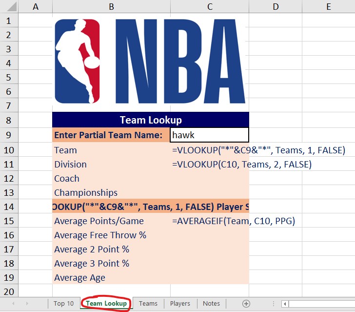
Step 4
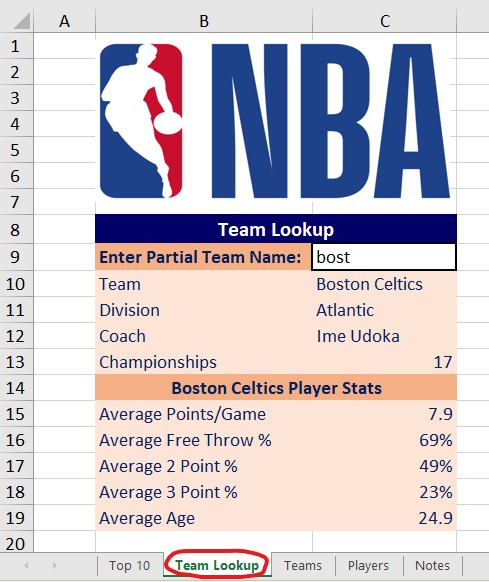
Create a new sheet named Team Lookup. It will have a cell where the user
can type the partial name of a team. It will lookup the full Team name,
Division, Coach, and Championships. It will show player statistics for the
team including Average Points/Game, Average Free Throw %, Average 2 Point %,
Average 3 Point %, and Average Age.
Create a named ranged called Teams: Select the Teams worksheet and select all (Ctrl-A). Click in the name box and enter Teams in the name box.
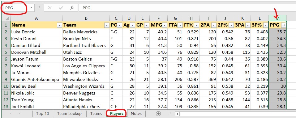
Create the PPG named ranged: Select the Players worksheet. Select the PPG column and enter PPG in the name box.
Select the Team Lookup worksheet. Here are some of the formulas to help you get started:
Cell C10: =VLOOKUP("*"&C9&"*",Teams,1,FALSE)
Cell C11: =VLOOKUP(C10,Teams,2,FALSE)
For the Coach and Championships, use the same formula as Division, but use 3 and 4 instead of 2 to pull from the 3rd and 4th columns.
Cell C15: =AVERAGEIF(Team,C10,PPG)